import numpy as np
import matplotlib.pyplot as plt
from scipy.optimize import curve_fit
from IPython.display import display, Markdown

1Pressure-Flow Relationships¶

The text mentions on page 16 that flow rate is proportional to pressure difference.

\frac{dV}{dt} \propto \Delta P

(1)

We can think about this as analogous to current flow in circuits. For example, $\Delta V$ is in units of Joules/Coulomb (energy per charge), while $\Delta P$ has units of Joules/ ${\rm m^3}$ (energy per volume). The volume in $\Delta P$ is whatever fluid is creating the pressure difference. If we consider the proportional relationship above and compare it to the proportional relationship that is Ohm’s Law, we have

Potential	Flow Rate	Proportionality
$\Delta V$	$I$	$R$
$\Delta P$	$\frac{dV}{dt}$	$R$

where we use $R$ as the constant of proportionality. You may already see that this constant is a resistance to flow in both cases.

Bernoulli’s Equation tells us that pressure throughout a fluid is constant.

P_1 + \rho gy_1 +\frac{1}{2}\rho v^2_1 = P_2 + \rho gy_2 +\frac{1}{2}\rho v^2_2

(2)

If the speed of fluid is small or nearly constant everywhere, we can ignore the dynamic term $\frac{1}{2}\rho v^2$ .

P_1 + \rho gy_1 = P_2 + \rho gy_2

(3)

Rearranging the equation,

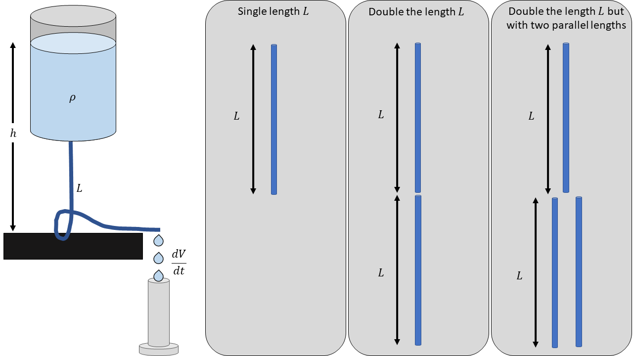
\begin{align} P_1 - P_2 &= \rho g\left(y_2 - y_1\right)\\ \Delta P &= \rho gh \end{align}

(4)

This says that pressure difference in a fluid can be considered as due to gravitational forces only when no other forces are present. In the following diagram, the pressure a hydrostatic water tower can be described by this equation.

Hydrostatic water tower diagram

In this system, there is a column of water $h$ high. The hydrostatic pressure is described by the equation above. The flow through the tube of length $L$ is described by

\Delta P = R\frac{dV}{dt}

(5)

1.1Experiment 1¶

We will do an experiment where we set $h$ , making it our independent variable. Thus, we will explore the relationship

\frac{dV}{dT} = \frac{\Delta P}{R}

(6)

To begin, measure the flow rate when there is a single length $L$ of tube, two lengths of tube in series $2L$ , and two lengths of tube but the second length has two parallel lengths. We will call the resistances $R_1$ , $R_{21}$ , and $R_{22}$ , for each scenario. Set $h=0.2~{\rm m}$ , and measure $dV/dt$ for these three scenarios. Record your results below and determine a relationship for $R_{21}$ and $R_{22}$ as a multiple of $R_1$ , e.g.,

R_{21} = n_{21}R_1

(7)

where $n$ is the multiple you are interested in finding.

p = #density of water (kg/m^3)
g = #acceleration due to gravity (m/s^2)
h = #depth of the water (m)

#use the values above to calculate pressure difference
DP = #pressure difference (Pascal)

dVdt1 = #flow rate of single tube (m^3/s)
dVdt21 = #flow rate of two tubes in series (m^3/s)
dVdt22 = #flow rate of two tubes with second tubes in parallel (m^3/s)

#use the values above to calculate resistances
R1 = 
R21 = 
R22 = 

#calculate the ratios to get n
n21 = 
n22 = 

#print the ratios
#This will print correctly if you calculate everything above correctly.
#Don't make changes below.
display(Markdown(
   rf"""
$n_{{21}}={n21}$

$n_{{22}}={n22}$
"""))

You should be able to convince yourself from the results that a particular length of the same kind of tubing (vessel) produces a particular amount of resistance. From electrical circuits that obey Ohm’s Law, we expect resistances in series to add

R_{\rm series} = R_1 + R_2 + R_3 + ... = \sum_i R_i

(8)

and in parallel, resistances add

R_{\rm parallel} = \left(\frac{1}{R_1} + \frac{1}{R_2} + \frac{1}{R_3} + ...\right)^{-1} = \left(\sum_i \frac{1}{R_i}\right)^{-1}

(9)

Does this agree with your results?

1.2Experiment 2¶

Let’s explore the relationships

\Delta P = \rho g h

(10)

and

\frac{dV}{dt} = \frac{\Delta P}{R}

(11)

We see from Experiment 1 that a certain type of tube (vessel) creates a certain resistance. If we attach a constant amount of tube, we should expect $R$ to be constant. Therefore, varying $h$ should affect the flow rate, and we can determine if there is a linear relationship between $\frac{dV}{dt}$ and $\Delta P$ .

Measure the flow rate for 4 different heights ranging from about 0.2 to 1.0 meters.
Enter the heights and flow rates below.
Calculate the pressure differences from the heights.
Plot flow rate vs. pressure difference.
Determine the resistance of the vessels.

# Enter data here
h = np.array([1,2,3,4])#enter the heights
dVdt = np.array([1,2,3,4])#enter the flow rates for each height (mL/s is fine.)
DP = # calculate the pressure differences (use p and g from above)

#Everything below should work without modification
#make a function for fitting data
def f_line(x, m, b):
    return m*x+b

#fit the data
fit_params, fit_cov = curve_fit(f_line, DP, dVdt, (1,0.1))
y_fit = f_line(DP, fit_params[0], fit_params[1])
print("slope = ", fit_params[0], "+/-", np.sqrt(fit_cov[0,0]))

plt.plot(DP, dVdt, 'ob', label="data")
plt.plot(DP, y_fit, '-k', label="fit")
plt.legend()
plt.xlabel(r'$\Delta P$ (Pa)')
plt.ylabel(r'$dV/dt$ (mL/s)')
plt.show()