print("Another code cell with a second optional metadata syntax")
In this chapter, we develop the tools to model the magnetic field that is produced by an electric current. We will introduce the Biot-Savart Law, which is analoguous to Coulomb’s Law in that it can be used to calculate the magnetic field produced by any current. We will also introduce Ampère’s Law, which can be thought of as the analogue to Gauss’ Law, allowing us to easily determine the magnetic field when there is a high degree of symmetry.
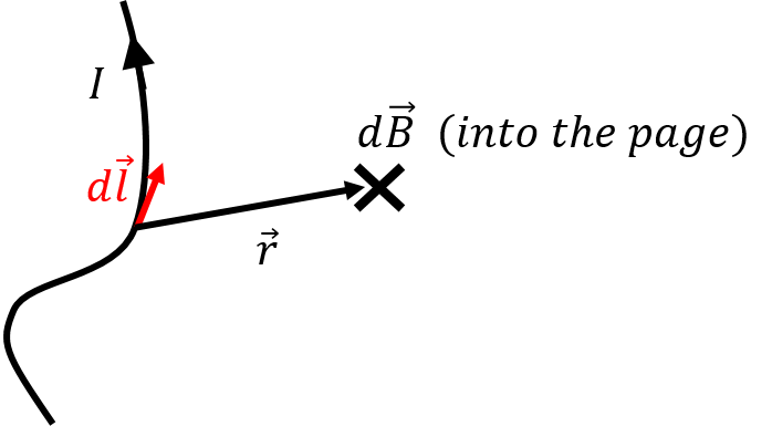
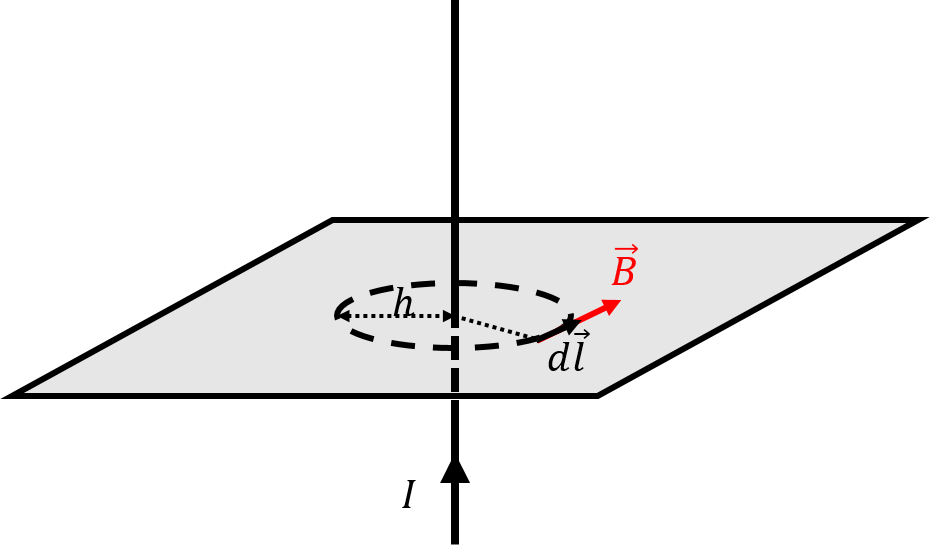
The Biot-Savart law allows us to determine the magnetic field at some position in space that is due to an electric current. More precisely, the Biot-Savart law allows us to calculate the infinitesimal magnetic field, dB, that is produced by a small section of wire, dl, carrying a current, I, such that dl is co-linear with the wire and points in the direction of the electric current:
where r is the vector from the element of wire, dl, to the point where we would like to determine the magnetic field, as illustrated in Figure 1. μ0 is a constant of proportionality called the “permeability of free space”, and has the value μ0=4π×10−7T⋅m/A.
Figure 1:The infinitesimal magnetic field, dB, that is created by an infinitesimal section of wire, dl, carrying current I. Note that the vector, r, goes from dl to the point where we wish to calculate the field.
The Biot-Savart Law has some similarities with the Coulomb Law to calculate the electric field, as the magnitude of the magnetic field decreases as the inverse of the square distance between the source and the field. However, it can only be expressed in differential form (i.e. as an infinitesimal) and it requires working in three dimensions because of the cross product. It is usually more convenient to use the Biot-Savart Law in the form:
The procedure for applying the Biot-Savart Law is as follows:
Make a really good diagram, as you will have to include some 3D aspects.
Choose an infinitesimal section of wire, dl.
Determine the vector r.
Determine the cross-product, dl×r, which will point in the direction of the magnetic field from that infinitesimal section of wire.
Write out the infinitesimal vector dB, and determine its components.
Think about symmetry! As you sum the dB, will some components cancel? If yes, you do not need to do those integrals.
Determine the total magnetic field, component by component, by summing (integrating) the components of dB over the wire.
21.2.1Magnetic field from a straight current-carrying wire
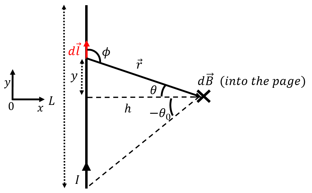
In this section, we use the Biot-Savart Law to determine the magnetic field a distance, h, from the centre of a finite straight wire of length L, carrying current I, as illustrated in Figure 2.
Figure 2:Setting up the model to use the Biot-Savart Law to calculate the magnetic field a distance h from the centre of a current-carrying wire of length L.
We start by choosing an infinitesimal element of wire, dl, a distance y above the centre of the wire, as shown (we choose the origin to be located at the centre of the wire). The vector dl is thus given by:
The cross-product between dl and r is easily found with the right-hand rule to point into the page (corresponding to the negative z direction). The magnitude of the cross-product is given by:
Any segment along the wire will result in a magnetic field that is into the page (negative z direction), thus there will be no cancellations due to any symmetries. We can now proceed to perform the integral.
We can use either θ or y to label the wire elements and carry out the integration. We will choose to integrate over θ, requiring us to express dl and r in terms of θ (and constants), as those are the only quantities in dB that depend on the position of dl. In order to express dl in terms of dθ, we first relate θ to y, the position of the wire element:
We define the angle, θ0, to be the maximum amplitude of the angle θ when integrating over the wire (see Figure 2), so that we integrate θ from −θ0 to +θ0:
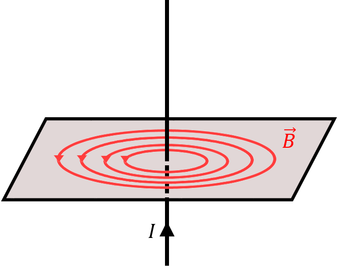
The magnetic field must be rotationally symmetric; that is, if the wire is vertical, the magnetic field at a distance h must look the same regardless of the angle from which we view the vertical wire (we should always see the magnetic field going into the page at the point that we use in Figure 2). Thus, the magnetic field lines must form circles around the wire, as illustrated in Figure 3. Note that the direction of the magnetic field is given by the right-hand rule for axial vectors; when you align your thumb with the current, your fingers curl in the direction of the magnetic field.
Figure 3:The magnetic field from a current-carrying wire forms concentric circles centred on the wire.
It is of particular interest to investigate the limiting case of an infinitely long wire, in the limit of L→∞, or equivalently, θ0→2π. The latter is easiest to evaluate, since sinθ0→1. The magnitude of the magnetic field, B, a distance, h, from an infinite wire carrying current, I, is given by:
One can often make the approximation that the wire is infinite in length, when the distance, h, is small compared to the length, L, of the wire.
21.2.2Magnetic field from a circular current-carrying wire
In this section, we examine the magnetic field that is created by a circular current-carrying loop of wire. We can determine the shape of the magnetic field, by considering small sections as straight wires, with circular magnetic field lines around them. As we move closer to the centre of the ring, those fields sum together, as illustrated in Figure 4. Note that the magnetic field from a loop of current is identical to that from a bar magnet (as a bar magnet is, of course, a collection of current loops).
Figure 4:The magnetic field from a current-carrying loop of wire can be thought of as the sum of the fields from small straight sections of wire.
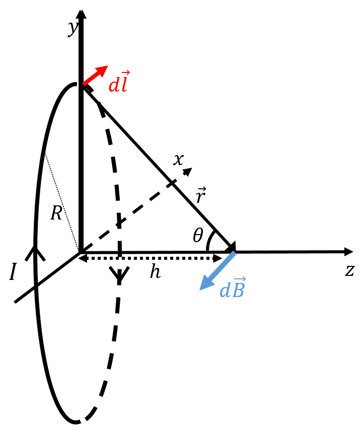
Below, we use the Biot-Savart Law to derive an expression for the magnitude of the magnetic field at a distance, h, from the centre of a ring of radius, R, along its axis of symmetry, when there is a current, I, in the ring. While the mathematics are much easier than the case for the straight wire, the challenge in this case is to visualize the calculation in three dimensions! Figure 5 shows the loop of current, as well as our choice of coordinate system (with the origin at the centre of the ring). In particular, we wish to calculate the magnetic field at a distance, h, along the z axis. The x axis goes into the page.
Figure 5:Diagram to apply the Biot-Savart Law in order to determine the magnetic field along the symmetry axis of a ring carrying current, I. The x axis goes into the page.
In order to apply the Biot-Savart Law, we choose an element, dl, of wire at the top of the ring, as illustrated. At this position, the element, dl, points in the positive x direction (into the page):
so that the element of magnetic field, dB, corresponding to that choice of dl, will lie in the y−z plane, as illustrated in Figure 5. Note that the vector dB is perpendicular to the vector r (since it is the cross-product of r with another vector). The magnetic field element, dB, is given by:
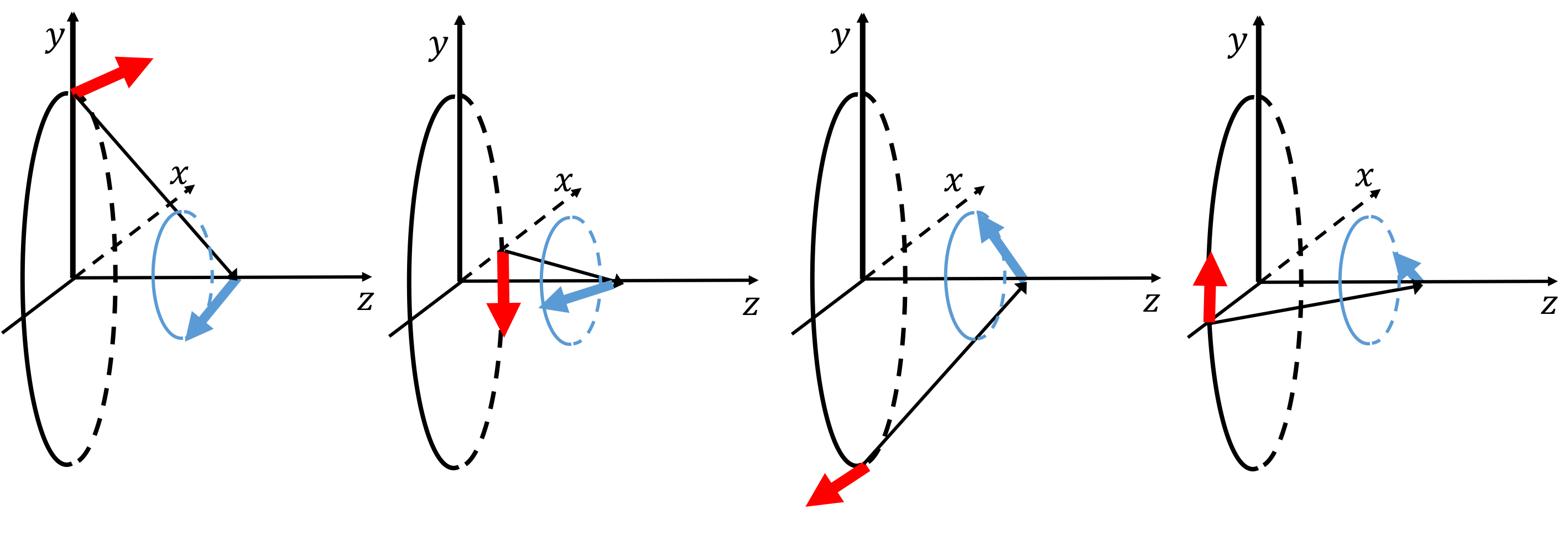
As the wire element, dl, moves around the circle, the tip of the resulting magnetic field vector element traces a circle centred on the z axis, as illustrated in Figure 6. Note that, in general, dB will also have an x component (the x component was only 0 before because we chose dl to be at the top of the ring). When we sum together the magnetic field elements, the x and y components will cancel, so that we are left with the z component.
Figure 6:As the wire element, dl, moves along the ring, the tip of corresponding magnetic field element vector, dB, describes a circle centred on the z axis. Thus, only the (negative) z component of dB will survive when these are all added together.
The total magnetic field will be in the negative z direction, as anticipated from Figure 4. Summing together the z components of the infinitesimal magnetic fields:
Note that in this case, both r and θ are constant for all of the dl, allowing us to take them out of the integral. The integral is then just a sum of the dl elements, which must add up to the circumference of the ring:
In this case, the math was relatively straightforward (no substitutions to evaluate the integral), however it is challenging to visualize the problem in three dimensions.
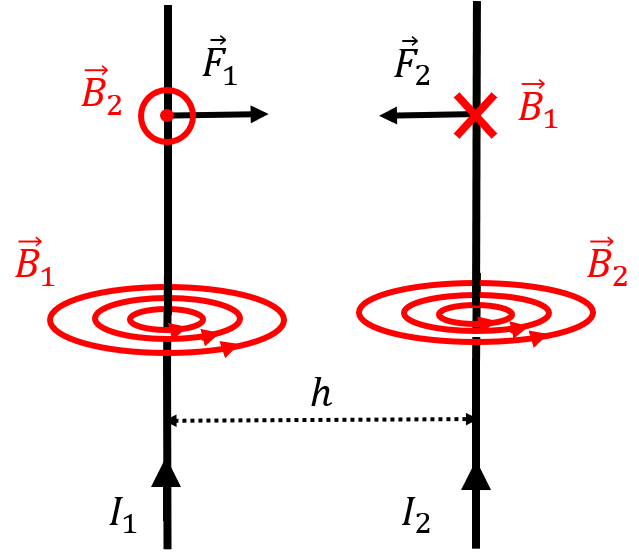
Consider two infinite parallel straight wires, a distance h apart, carrying upwards currents, I1 and I2, respectively, as illustrated in Figure 7.
Figure 7:Two parallel current-carrying wires will exert an attractive force on each other, if their currents are in the same direction.
The first wire will create a magnetic field, B1, in the shape of circles concentric with the wire. At the position of the second wire, the magnetic field B1 is into the page, and has a magnitude:
Since the second wire carries a current, I2, upwards, it will experience a magnetic force, F2, from the magnetic field, B1, that is towards the left (as illustrated in Figure 7 and determined from the right-hand rule). The magnetic force, F2, exerted on a section of length, l, on the second wire has a magnitude given by:
where we used the fact that the angle between l and B is 90°. We expect, from Newton’s Third Law, that an equal and opposite force should be exerted on the first wire. Indeed, the second wire will create a magnetic field, B2, that is out of the page at the location of the first wire, with magnitude:
This leads to a magnetic force, F1, exerted on the first wire, that points to the right (from the right-hand rule). On a section of length, l, of the first wire, the magnetic force from the magnetic field, B2, has magnitude:
which does indeed have the same magnitude as the force exerted on the second wire. Thus, when two parallel wires carry current in the same direction, they exert equal and opposite attractive forces on each other.
The attractive force between two wires used to be the basis for defining the Ampère, the S.I. (base) unit for electric current. Before 2019, the Ampère was defined to be “that constant current which, if maintained in two straight parallel conductors of infinite length, of negligible circular cross-section, and placed one metre apart in vacuum, would produce between these conductors a force equal to 2×10⁻¹⁷N per metre of length”. Recently, the definition was updated to be based on defining the Coulomb in such a way that the elementary charge has a numerical value of e=1.602176634×10⁻¹⁹C, and the Ampère corresponds to one Coulomb per second.
The force between two wires is a good system to understand how any physical quantity cannot depend on our choice of the right-hand to define cross-products. As mentioned in the previous chapter, any physical quantity, such as the direction of the force exerted on a wire, will always depend on two successive uses of the right hand. In this system, we first used the right-hand rule for axial vectors to determine the direction of the magnetic field from one of the wires. We then used the right-hand rule to determine the direction of the cross-product to determine the direction of the force on the other wire. You can verify that you get the same answer if you, instead, use your left-hand to define the direction of the magnetic field (which will be in the opposite direction), and then again for the cross-product. This also highlights that the magnetic field (and the electric field) is just a mathematical tool that we use to, ultimately, describe the motion of charges or compass needles.
Ampère’s Law is similar to Gauss’ Law, as it allows us to (analytically) determine the magnetic field that is produced by an electric current in configurations that have a high degree of symmetry. Ampère’s Law states:
where the integral on the left is a “path integral”, similar to how we calculate the work done by a force over a particular path. The circle sign on the integral means that this is an integral over a “closed” path; a path where the starting and ending points are the same. Ienc is the net current that crosses the surface that is defined by the closed path, often called the “current enclosed” by the path. This is different from Gauss’ Law, where the integral is over a closed surface (not a closed path, as it is here). In the context of Gauss’ Law, we refer to “calculating the flux of the electric field through a closed surface”; in the context of Ampère’s Law, we refer to “calculating the circulation of the magnetic field along a closed path”.
We apply Ampère’s Law in much the same way as we apply Gauss’ Law:
Make a good diagram, identify symmetries.
Choose a closed path over which to calculate the circulation of the magnetic field (see below for how to choose the path). The path is often called an “Amperian loop” (think “Gaussian surface”).
Evaluate the circulation integral.
Determine how much current is “enclosed” by the Amperian loop.
Apply Ampère’s Law.
Similarly to Gauss’ Law, we need to choose the path (instead of the surface) over which we will evaluate the integral. The integral will be easy to evaluate if:
The angle between B and dl is constant along the path, so that:
Choosing a path that meets these two conditions is only possible if there is a high degree of symmetry.
Consider an infinitely long straight wire, carrying current, I, out of the page, as illustrated in Figure 10. The magnetic field from the wire must look the same regardless of the angle from which we view the wire (“azimuthal symmetry”). Thus, the magnetic field must either form concentric circles around the wire (which we know is the case from the Biot-Savart Law) or it must be in the radial direction (pointing towards or away from the wire). These two possibilities are illustrated in Figure 10, and we will pretend, for now, that we do not know which is correct.
Figure 10:By symmetry, the magnetic field from a current-carrying infinite wire (illustrated with current coming out of the page), must either form concentric circles (left panel), or be in the radial direction (right panel). We know that the former (circles, left panel) is the correct choice. The dotted lines show “Ampèrian loops” that one can use to calculate the integral in Ampère’s Law.
In order to apply Ampère’s Law, we choose an Amperian loop (instead of a “Gaussian surface”). In the case of an infinite current-carrying wire, a circle that is concentric with the wire will meet the properties above, regardless of the two possible configurations of the magnetic field: with a circular Amperian loop, the angle between the magnetic field and the element dl is constant along the entire loop, and the magnitude of the magnetic field is constant along the loop. Our choice of loop is illustrated in Figure 11, where we have illustrated the magnetic field for the case where it forms concentric circles.
Figure 11:An Amperian loop that is a circle of radius, h, will allow us to determine the magnetic field at a distance, h, from an infinitely-long current-carrying wire.
The circulation of the magnetic field along a circular path of radius, h, is given by:
where cosθ is 1 if the field forms circles (correct) or 0 if the field is radial (incorrect). We can now evaluate the current that is enclosed by the Amperian loop. The current that is enclosed is given by the net current that traverses the surface defined by the Amperian loop (in this case, a circle of radius h). Since the loop encloses the entire wire, the enclosed current is simply I. Applying Ampère’s Law:
At this point, it is clear that cosθ cannot be zero, since the right-hand side of the equation is not zero. We can thus conclude that the magnetic field must indeed make concentric circles, as we had previously determined. The magnitude of the magnetic field is given by:
as we found previously with the Biot-Savart Law. Again, in analogy with Gauss’ Law, one needs to apply some knowledge of symmetry and argue in which direction the magnetic field should point, in order to use Ampère’s Law effectively.
21.4.1Interpretation of Ampère’s Law and vector calculus
In this section, we discuss Ampère’s Law in the context of vector calculus and provide a different perspective, mostly for informational purposes. The integral that appears in Ampère’s Law is called the “circulation” of the vector field, B:
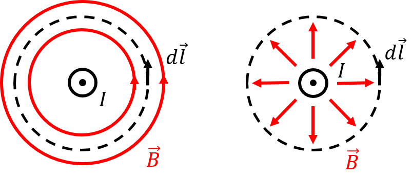
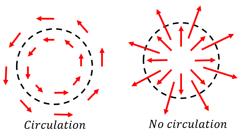
The circulation, as its name implies, is a measure of “how much rotation there is in the field”. To visualize this, imagine that the vector field is a velocity field for points in a fluid. Regions of the fluid where there are little whirlpools (so called “eddies”), correspond to regions of the field with non-zero circulation (the sign of the integral tells us the direction of rotation, using the right-hand rule for axial vectors). Examples of field with and without circulation are shown in Figure 14. You will recognize that static electric charges create electric fields with no circulation (right panel), whereas static currents create magnetic fields with circulation.
Figure 14:Examples of field with (left panel) and without (right panel) circulation, as evaluated along the closed loop shown with the dashed line.
Ampère’s Law is thus a statement that an electric current will result in a field with a magnitude proportional to the current, that has some degree of rotation to it. The direction of rotation of that field corresponds to the right-hand rule for axial vectors as applied to the current (your thumb points in the direction of the current so that your fingers curl in the direction of the rotation of the associated field).
Circulation, as defined by the integral over a closed loop, is not a local property of the field, since it depends on what the field is doing as a whole over the path of the loop. Just as one can obtain a “local” version of Gauss’ Law, one can also obtain a local version of Ampère’s Law using techniques from advanced vector calculus (that are beyond the scope of this textbook).
Stokes’ theorem allows one to convert the circulation integral (a path integral on a closed loop) into a integral over the (open) surface that is defined by the loop:
where the subscript C indicates that the integral is over a one-dimensional path, whereas the subscript S indicates that the integral is over a two-dimensional surface. The term, ∇×B, is called the “curl” of the magnetic field and is a local measure of the amount of rotation in the field. Applying Stokes’ theorem to Ampère’s Law yield:
Note that we can also write the current, Ienc, that is enclosed by the loop as the integral of the current density, j, over the surface defined by the loop:
This last equation now relates a local property (current density) to the magnetic field at that point, and is the usual form in which Ampère’s Law is presented (the so-called “differential form”, rather than the “integral form”).
The curl of the magnetic field, ∇×B, is a vector that is given by the following:
and the name “curl” is chosen because this is a measure of the amount of rotation (curl) in the field. In differential form, Ampère’s Law can read as: “a current density will create a (magnetic) field that has non-zero curl”.
Since Ampère’s Law in differential form is a vector equation (both sides are vectors), it really corresponds to three equations in Cartesian coordinates, one per component. For example, the x component of the equation is a “partial differential equation” for the y and z components of the magnetic field:
that is in general difficult to solve without a computer (and all three equations are required, as these are “coupled”, since a given component of the magnetic field appears in two of three equations).
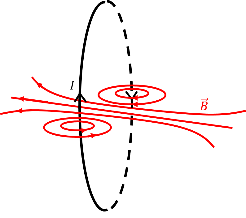
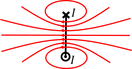
In order to create strong magnetic fields, the most practical method is to combine many loops of current together into a “solenoid” (a coil). Electromagnets function on this principle and are ubiquitous in our lives. Figure 15 shows the magnetic field from a single loop of current.
Figure 15:The magnetic field from a single loop of current.
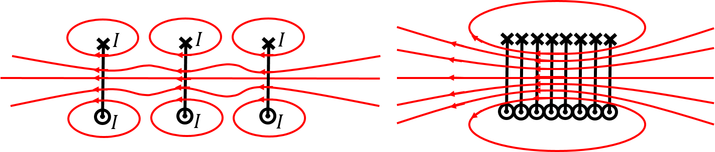
When several loops of current are brought close together, as in Figure 16, the magnetic field inside the solenoid becomes uniform, and the magnetic field just outside the solenoid approaches zero.
Figure 16:As multiple loops of current are brought together to form a solenoid, the magnetic field inside the solenoid becomes uniform and the field outside the solenoid approaches zero.
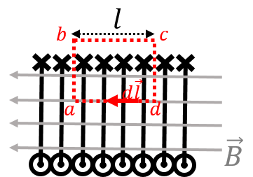
We can use Ampère’s Law to determine the strength of the magnetic field inside of a solenoid, under the assumption that the magnetic field is uniform in the volume of the solenoid and zero just outside. Consider a solenoid with current, I, going through it, that contains n loops per unit length. In order to determine the magnetic field, B, inside of the solenoid, consider the rectangular Amperian loop, abcd, of length, l, illustrated in Figure 17.
Figure 17:We use Ampère’s Law with a rectangular loop to evaluate the strength of the magnetic field inside a solenoid.
In order to evaluate the circulation of the magnetic field around the loop, abcd, we divide the loop up into segments, and evaluate the path integral (∫B⋅dl) over each segment, then add those together to obtain the integral over the closed path:
Over each segment, the vector dl will be parallel to that segment. Only the last term is non-zero. The integrals over the segments ab and cd are zero because the magnetic field is perpendicular to dl over those segments (so the scalar product is zero). The integral over the segment bc is zero because the magnetic field is zero just outside the solenoid. The integral over the last segment, where dl and B are parallel, is simply given by:
since the length of the segment is l, and the magnetic field is constant in magnitude.
In order to apply Ampère’s Law, we must determine the current that is enclosed by our Amperian loop. Since the rectangular loop has a length, l, it will enclose N=nl loops of current, I, since there are n loops per unit length. Thus the enclosed current is Ienc=nlI. Applying Ampère’s Law, we find the magnetic field inside a solenoid:
which does not depend on our (arbitrary) choice of making an Amperian loop with an arbitrary length of l. In practice, when solenoids are used as electromagnets, they are typically filled with a ferromagnetic material, which will magnetise when there is a current, resulting in a stronger magnetic field. This is usually done by winding a wire around an iron rod.
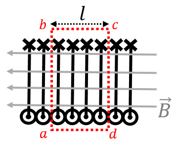
Note that if we extend the Amperian loop so that the bottom segment is also outside the solenoid, as in Figure 18, it is easy to show that the magnetic field immediately outside of the solenoid must be zero. Indeed, in this case, there are an equal number of currents coming out of the page as there are going into the page, so that the net current that is enclosed by the Amperian loop (the net current that crosses the plane of the loop) is identically zero, so that the circulation must be zero, implying that the magnetic field is zero just outside the solenoid.
Figure 18:By extending the Amperian loop to both sides of the solenoid, we conclude that the magnetic field just outside the solenoid must be zero, because the net current enclosed is zero.
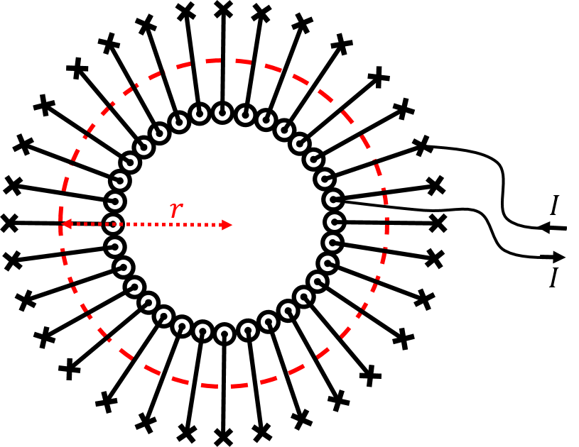
A toroid can be thought of as a solenoid that has been bent into the shape of a circle (or rather, a torus), as illustrated in Figure 19. Inside the toroid, the magnetic field forms concentric circles (not shown).
Figure 19:An Amperian loop of radius r to determine the magnetic field inside of a toroid. Note that the magnetic field everywhere outside the toroid must be zero (think of the current enclosed by Amperian loops).
Again, we can use Ampère’s Law to determine the strength of the magnetic field inside the toroid. Consider the circular Amperian loop of radius r that is illustrated in Figure 19. Since the magnetic field is parallel to the Amperian loop everywhere along the loop, and the magnetic field does not change magnitude (by symmetry), the circulation is given by:
If the toroid contains N loops of current, then the enclosed current is given by Ienc=NI, since the Amperian loop include N times the current I coming out of the page. Ampère’s Law thus gives the magnitude of the magnetic field as:
which decreases in magnitude with increasing radius, as long as we are inside the toroid. It is easy to show, by using Amperian loops that are either smaller or bigger than the toroid, that the magnetic field everywhere outside of the toroid is exactly zero (as those Amperian loops will enclose no net current). In a toroid, the magnetic field lines form closed circles. For a solenoid, there must exist a magnetic field somewhere outside the solenoid, in order for the field lines inside the solenoid to close. We can usually ignore these if the solenoid is long, as the field outside will be very weak, and very close to zero very close the solenoid (as we showed with Ampère’s Law above).
Magnetic fields are created by moving charges. The Biot-Savart Law allows us to determine the infinitesimal magnetic field, dB, that is produced by the current, I, flowing in an infinitesimal section of wire, dl:
where μ0 is a constant called the permeability of free space. The vector r points from the wire element, dl, to the point at which we want to determine the magnetic field. In order to determine the magnetic field from a finite wire, one must sum (integrate) the contributions that come from each section of wire. It is often easier to work with the Biot-Savart law written without the unit vector, r^:
The magnetic field from a straight current-carrying wire forms concentric circles centred around the wire. The direction of the magnetic field is given by the right-hand rule for axial vectors; with the thumb pointing in the direction of current, the fingers curl in the direction of the magnetic field.
The magnitude of the magnetic field, a distance, h, from the centre of a circular loop of wire with radius, R, carrying current, I, along the axis of symmetry of the loop is given by:
The direction of the magnetic field can also be found using the right-hand rule for axial currents. In this case, if your fingers curl in the direction of the current loop, your thumb points in the same direction as the magnetic field at the centre of the loop.
Two parallel wires carrying currents, I1 and I2, separated by a distance, h, will exert equal and opposite forces on each other with a magnitude:
The force is attractive if the two currents flow in the same direction and repulsive otherwise.
Ampère’s Law is the magnetism analogue to Gauss’ Law. Just like Gauss’ Law, it requires a high degree of symmetry to be applied analytically, although it is always valid. Ampère’s Law relates the circulation of the magnetic field around a closed path to the current enclosed by that path:
In order to apply Ampère’s Law, we must first choose an Amperian loop over which to compute the closed path integral (instead of choosing a Gaussian surface to calculate the flux of the electric field on a closed surface). The circulation integral will be straightforward to evaluate if:
The angle between B and dl is constant along the path, so that:
The current enclosed, Ienc, corresponds to the net current that crosses the surface that is defined by the Amperian loop (a closed path always defines a surface).
Ampère’s Law is straightforward to use in situations with a high degree of symmetry, such as infinitely long wires carrying current.
Solenoids are formed by combining many loops of current together, in order to form a strong and uniform magnetic field. The magnetic field inside of a solenoid has a magnitude of:
where, I, is the current in the solenoid, and n, is the number of loops per unit length in the solenoid. The magnetic field just outside of a solenoid is zero, and generally, the magnetic field is negligible outside of a solenoid.
A toroid is formed by bending a solenoid into a circle to form a torus. The magnetic field lines inside of a toroid form concentric circles. The magnetic field decreases with radius inside of a toroid and is identically zero everywhere outside a toroid.
The square loop is simply made of four straight sections of wire of length, L. The magnetic field from each section of wire is into the page, which you can easily verify with your right-hand (with your thumb in the direction of current, your fingers curl in the direction of the resulting magnetic field).
The magnetic field at the centre is just four times the magnetic field produced by a single segment, which we determined in this chapter. The magnetic field at the centre of the loop is thus four times the magnetic field at a distance, h=2L, from a wire of length, L:
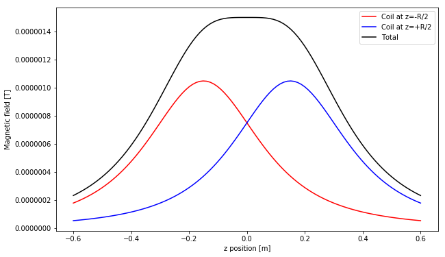
For the two coils in the Helmholtz configuration, the magnetic field from each coil will be in the same direction. The centre of the two coils are located at z=±2R. Thus, if we are located at position, z, along the z axis, one coil will be at a distance of z+2R, and the other at a distance z−2R. The total magnetic field as a function of z is then given by:
We can plot this function, as well as the two individual terms using python. For information, we show the code below. In order to make the plot, we need to choose some reasonable values for the radius of the coils and the current through the coils, for example:
R=0.3m
I=0.5A
#Import the modules that we need:
import numpy as np
import matplotlib.pyplot as plt

#Define some constants:
mu0 = 4*np.pi*1e-7 #4 pi
I = 0.5
R = 0.3

#Define the values on the z axis, from -2R to +2R, in 100 increments
z = np.linspace(-2*R,2*R,100)

#Determine the magnetic field from the coils at those values of z
#The coil at z = - R/2:
B1 = (mu0*I)/2 * R**2/((R**2+(z+R/2)**2)**(3/2))
#The coil at z = + R/2:
B2 = (mu0*I)/2 * R**2/((R**2+(z-R/2)**2)**(3/2))
#The sum:
B = B1 + B2

#Make the plot
plt.figure(figsize=(10,6))
plt.plot(z,B1,label='Coil at z=-R/2')
plt.plot(z,B2,label='Coil at z=+R/2')
plt.plot(z,B,label='Total')
plt.legend()
plt.xlabel('z position [m]')
plt.ylabel('Magnetic field [T]')
plt.show()
Figure 22:Magnetic field from each coil, as well as their sum, for two coils in the Helmholtz configuration
As advertised, we see a region between the Helmholtz coils where the magnetic field is nearly uniform.