Overview
Introduction
Producing electronic signals for circuits and measuring input and output signals of electronics circuits is important for a wide variety of applications. Everything from power lines to cell phones to Fitbits use electronic signals and circuits. This lab will explore signals and their measurement. We will use a FeelTech FY3200S Figure 1 signal generator capable of producing alternating signals in sine, square, triangle, and arbitrary formats. We will use a Tektronix TBS 1072B-EDU Figure 2 digital oscilloscope to measure the waveforms from the signal generator (input) and from simple circuits (output).
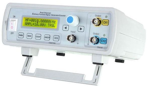
Figure 1:The FeelTech FS3200 signal generator.
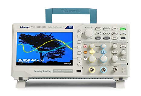
Figure 2:The Tektronix 1102BEDU oscilloscope.
Part 1 of this lab is to familiarize yourself with the signal generator and the oscilloscope.
Part 2 of this lab is to measure the output impedance of the FeelTech signal generator. The output impedance is a measure of the source’s propensity to drop in voltage when the load draws current, the source being the portion of the circuit that transmits and the load being the portion of the circuit that consumes. Because of this the output impedance is sometimes referred to as the source impedance or internal impedance.
Part 3 of this lab is to measure the integrity of the signal generator. We will do this by looking at the accuracy of the frequency and the rise time of a square wave.
Experiment
Part 1 - Familiarizing with the Equipment
Explore the signal generator.
Set up a signal generator and oscilloscope as shown in Figure 3. The equivalent circuit you are measuring is shown in . The output of the signal generator CH1 should be a 2 Volt peak-to-peak sine wave with a frequency of 1000 Hz. Connect a BNC to alligator clip cable to CH1 on the signal generator (yellow). Connect a BNC to alligator clip to the oscilloscope channel 1 (yellow). Use the alligator clips to connect a 100Ω load resistor.

Figure 3:The setup of the experiment. A signal generator connected to a load. The oscilloscope measures the voltage signal across the load. The load signal would be equal to the signal generator signal if there were no output impedance.

Figure 4:Equivalent circuit showing a sine wave going through two resistors in series. The oscilloscope measures the voltage across the load, indicated by the circles.
Explore the oscilloscope
When you have your circuit connected, try to find the signal on the oscilloscope.
Part 2 - Signal Generator Output Impedance
Measurements
Use at least 10 different load resistors between 10 and 100 000 to measure . For such a large range, it is useful to use a logarithmic scaling such as the load resistor values in Table 1. This logarithmic scaling uses three values per power of ten, or per decade, that are nearly evenly spaced on a log scale.
Figure 3 and show the circuit you will be analyzing. The output impedance (resistance) of the signal generator is fixed by the signal generator. All instruments have such an impedance, and it may be important to know its value depending on the electronics work you are doing. It is difficult to characterize a single resistance in a circuit, and therefore, we will rely on the voltage divider circuit discussed in Part 4 - Application: Voltage Divider to Measure Temperature.
Table 1:Resistor values separated logarithmically over five decades.
| decade | values |
|---|---|
| 10 | 10, 20, 50 |
| 100 | 100, 200, 500 |
| 1000 | 1000, 2000, 5000 |
| 10 000 | 10 000, 20 000, 50 000 |
| 100 000 | 100 000 |
Theory
According to Ohm’s Law, we know
We know from the equivalent circuit that the series resistance is
We also know for series resistors, the voltages sum to the input voltage
Finally, we know the current is the same throughout the circuit.
Analysis
Enter your data into the arrays and make a graph for part 1 using the Python code shown below. You have a list of values for the load resistor Rload, the voltage on the load resistor Vload, and uncertainties for both of these lists Rload_unc and Vload_unc. The uncertainty for the load resistor can be from the silver (10%) or gold (5%) band on the resistors you used.
import numpy as np
import matplotlib.pyplot as plt
from scipy.optimize import curve_fit

#define a linear function
def line_fit (x, m, b):
	return m*x + b

#Define your data
Rload = np.array([10., 15., 27., 33., 47., 68., 100., 150., 330., 470., 680., 1000., 10000., 22000.])
Rload_unc = 0.05*Rload #gold band resistors
Vload=np.array([0.38, 0.52, 0.74, 1.08, 1.02, 1.20, 1.40, 1.56, 1.84, 1.88, 1.94, 1.98, 2.06, 2.08])
Vload_unc = np.array([0.1,0.1, 0.1, 0.1, 0.1, 0.1, 0.1, 0.1, 0.1, 0.1, 0.1, 0.1, 0.1, 0.1])

#Do the linear fit
parms, cov = curve_fit(line_fit, 1/Rload, 1/Vload, sigma=Vload_unc, absolute_sigma=True)
print("slope=", parms[0], +/-", np.sqrt(cov[0,0])
print("intercept=", parms[1], +/-", np.sqrt(cov[1,1])

plt.errorbar(1/Rload, 1/Vload, yerr=Vload_unc/Vload**2, fmt='ob') #plot the data
plt.plot(1/Rload, parms[0]*1/Rload+parms[1])
plt.xlabel(r'$1/R_{load}$')
plt.ylabel(r'$1/V_{load}$')
plt.show()Part 3 - Signal Integrity
Experiment
Determine the accuracy of the frequency of the signal generator as a function of frequency. For a sine wave and a square wave of 2 Volts peak-to-peak, adjust the frequency using a log-scale, i.e., 10 Hz, 20 Hz, 50 Hz, 100 Hz, 200 Hz, 500 Hz, etc. up to 10 MHz. Record the signal generator frequency as your x-value and the oscilloscope value as your y-value. You will have two datasets, one for sine and one for square. Keep in mind you will need to adjust the horizontal scaling on the oscilloscope so that you can see at least one period of the wave. The oscilloscope will measure the frequency and period for you. However, you should include in your report how you can use the screen and scaling adjustments to get an accurate measurement manually.
When measuring the square wave, use the cursor capabilities on the oscilloscope to measure the time it takes the square wave to go from its highest to lowest point on the falling side of the square wave. We’ll call this the “fall time”.
Analysis
Enter your data into the arrays of the code below and make three graphs for part 2. The first graph is done for you.
Graph 1 - Sine Wave
For the first graph of the sine function, you have a list of values for the signal generator frequency signal_f, the measured signal frequency on the oscilloscope oscope_f, and uncertainties for the oscilloscope measurement oscope_f_unc. These uncertainties will need to be estimated based on the oscilloscope settings. You will want to plot these values on a log-log scaled graph. To do this, use plt.errorbar(np.log(oscope_f), np.log(signal_f), yerr=oscope_f_unc)Add a linear trendline to this data.
Graph 2 - Square Wave You have the same data for the square wave. Create a graph of measured frequency vs. signal frequency with a linear fit.
Graph 3 - Fall Time
For the fall time, you have signal_f, fall_time, and fall_time_unc.
signal_f = np.array([10, 100, 1000, 10000, 100000, 1000000, 10000000])
oscope_f_sine = np.array([10.001, 100.002, 1000.01, 10000, 100000, 1000010, 10000000])
oscope_f_sq = np.array([10.0000, 100.000, 1000.01, 10000, 100000, 1000000, 10000000])
fall_time = np.array([41, 41, 37, 37, 40, 40, 51])

#define a linear function
def line_fit (x, m, b):
	return m*x + b

#Do the linear fit
parms, cov = curve_fit(line_fit, signal_f, oscope_f_sine)
print(parms, np.sqrt(cov))

plt.plot(np.log(signal_f), np.log(oscope_f_sine), 'ob') #plot the data
plt.plot(np.log(signal_f), np.log(parms[0]*signal_f+parms[1]))
plt.xlabel('Signal Generator Fequency (Hz)')
plt.ylabel('Oscilloscope Frequency (Hz)')
plt.show()